LESSON 8 MEASURES OF CENTRAL TREND, POSITION AND DISPERSION.
They apply only to quantitative variables.
1. NUMERICAL SUMMARY OF A
STATISTICAL SERIES.
There are three major types of statistical measures:
- Measures of position: idea of the magnitude, size of the position of
observations of the data once they are ordered from minor to a mayor.
- Measures of central tendency: idea of the central behavior of the
subjects.
- Measures of dispersion or variability: information about the
heterogeneity of subjects, ie whether they are very different from each other
or not.
They only apply to continuous quantitative variables.
2. CENTRAL TREND MEASURES
• Arithmetic mean or mean: for quantitative variables.
It is calculated for quantitative variables and is the geometric or gravity
center of our data.
When the data are grouped
(two intervals), to calculate the mean we use as reference value of each
interval its class mark: we calculate a weighted arithmetic mean that is
obtained by summing the class mark by the absolute frequency, between N.
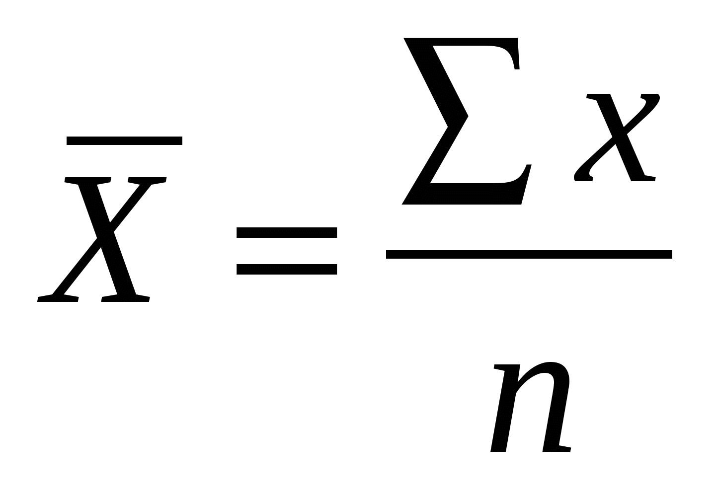
- x= Ʃmc (mark of class) fi /n (We multiply the mark of class by the absolute frequency and we are adding, then we divide between the number of subjects)
- Median: Value that occupies the center position in an ordered list of data.
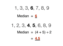
• Property: robustness. It only takes into account the position of the values in the sample and therefore has much better behavior than the average when there are extreme observations.
• Mode: It is the value most frequently (which is repeated
more times). If there is more than one, the sample is said to be bimodal (two
fashions) or multimodal (more than two fashions). Any qualitative or
quantitative variable can be calculated for any type of variable.

3. POSITION OR QUANTITY MEASURES
They are calculated for quantitative variables and, like the median, only take into account the ordered position of greater or lesser values in the sample. The most common quantiles are percentiles, deciles, and quartiles, as they divide the ordered sample into 100 (perciles), 10 (deciles), or 4 parts (quartiles), respectively.
- Percentiles: Divide the
ordered sample into 100 parts. The value of P50 corresponds to the median
value.
- Deciles: Divide the ordered
sample into 10 parts. The value of D5 corresponds to the value of the median
and, therefore, the value of the P50.
- Quartile: Divide the
ordered sample into 4 parts.


4. DISPERSION MEASURES
The information provided by the measures of central tendency is limited.
Example:
- Series 1: 18, 19, 20, 21, 22. (the first group is homogeneous because
they have the closest ages)
- Medium series 1 = 20
- Series 2: 9, 14, 20, 27, 30.
- Medium series 2 = 20
What differentiates one from the
other? The dispersion.
• Range or path: Difference
between the highest and lowest value of the sample lXn-X1l (absolute value).
According to the previous example:
- R1 = 22-18 = 4
- R2 = 30-9 = 21 (this already indicates to us that the series 2 has more
dispersion).


• Mean deviation: Arithmetic mean of the distances of each observation with
respect to the sample mean:


• Standard or Standard Deviation:
Quantifies the error we make if we represent a sample solely by its mean. This
is the one that is most used because it gives us a greater range of error:


• Variance: Express the same information in quadratic values:

• Interquartile range: Difference between the third and the first quartile = lQ3-Q1l
-
Coefficient of variation: It is a
measure of relative dispersion (dimensionless). It serves us to compare the
heterogeneity of two numerical series independently. It goes from 0 to 1.

5. NORMAL DISTRIBUTIONS
In statistics is called
normal distribution, Gaussian distribution or Gaussian distribution, to one of
the distributions of probability of continuous variable that more frequently
appears in real phenomena. The normal distributions in a histogram show the
Gaussian bell. And it is symmetrical with respect to the values of central
position, that is to say that the fashion will coincide with the mean and the
median.
6.
ASYMMETRY AND KURTOSIS


• Asymmetry
coefficient of a variable: Asymmetry degree of the distribution of its data
around its mean, the more asymmetric it is, the more different values we will
find.
Asymmetries:
The results can be as follows:
- g1
= 0 (symmetric
distribution; there is the same concentration of values to the right and left
of the mean).
- g1> 0
(positive asymmetrical distribution, there is a higher concentration of values
to the right of the mean than to its left).
- g1
<0 (negative asymmetric
distribution; there is a higher concentration of values to the left of the
mean than to the right).
• Kurtosis or pointing of the curve: It has no relation to symmetry. It serves to measure the degree of concentration of the values it takes around its mean. The data accumulates a lot. A variable with normal distribution is chosen as reference, so that for it the kurtosis coefficient is 0.
The results can be as follows:
- g2
= 0 (mesocuric or normal
distribution). It has a mean degree of concentration around the central values
of the variable (the same that has a normal distribution).
-
g2> 0 (leptokurtic
distribution). It presents a high degree of concentration around the central
values of the variable.
- g2
<0 (platicurtic
distribution). It presents a reduced degree of concentration around the central
values of the variable.

We work with a continuous variable that:
- Follows a normal distribution (TLC)
- It has more than 100 units (LGN)
The typing allows us to know if value corresponds or not
to that distribution frequently
We know from the shape of the curve that:
The average matches the top of the bell: 8
The standard deviation is 2 points:
- 50% have scores> 8 - 50% have scores <8
- Approximately 68% score between 6 and 10
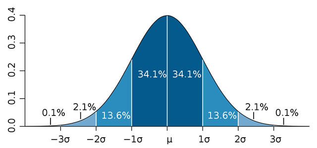
- 50% have scores> 8 - 50% have scores <8
- Approximately 68% score between 6 and 10
No hay comentarios:
Publicar un comentario